FMI Layered Standard for DAE (FMI-LS-DAE)

This layered standard on top of FMI 3.0 defines how to exchange dynamic models in differential algebraic equation form.

Although the document refers to version 3.0 of the FMI standard, everything described in this document also applies to all subsequent minor versions. For further information on compatibility, see section Versioning and Layered Standards in the FMI 3.0 specification.

This document is licensed under the Attribution-ShareAlike 4.0 International license. The code is released under the 2-Clause BSD License. The license text can be found in the LICENSE.txt file that accompanies this distribution.

1. Introduction

1.1. Intent of this Document

A differential-algebraic system of equations (DAE) is a system of equations that either contains differential equations and algebraic equations, or is equivalent to such a system ^[1].

Avoid the requirement of index reduction inside of FMUs.
- This could improve accuracy due to better drift handling.
Avoid local nonlinear equation solvers inside of FMUs.
- This could improve accuracy and avoid problems with different local and global error tolerances.
Preserve the sparseness of DAE systems which is lost for the corresponding reduced ODE systems.
- This could improve the performance by usage of the sparseness.
Allow connections between constraint FMUs.
- Connecting reduced ODE FMUs could lead globally to a non-solvable (singular) system but not for unreduced DAE FMUs.

1.2. How to read this Document

The standard document is in HTML allowing heavy use of in-document links: all state names, function names, many function arguments, XML elements and attributes are links to definitions or descriptions.

In key parts of this document, non-normative examples are used to help understand the standard.

Conventions used in this document:

Non-normative text is given like this:

Especially examples are defined in this style.
The key words "MUST", "MUST NOT", "REQUIRED", "SHALL", "SHALL NOT", "SHOULD", "SHOULD NOT", "RECOMMENDED", "MAY", and "OPTIONAL" in this document are to be interpreted as described in RFC 2119 (regardless of formatting and capitalization).
State machine states are formatted as bold link, e.g. InitializationMode.

1.3. Overview

2. Common Concepts

2.1. Mathematical Notation

Table 1. Additional symbols for specific variable types.
Variable	Description
$\mathbf{z}_c$	A vector of real continuous-time variables representing the continuous-time algebraic variables.

2.1.1. DAE representation

There are different forms of DAEs.

For simplicity discontinuous states are currently disregarded.

2.1.1.1. Fully-Implicit DAE

The generic fully-implicit DAE, or implicit DAE, formulation:

\[F(\dot{z}(t), z(t), t) = 0\]

where $z(t)$ represents state and additional variables and $t$ is time.

A similar and sometimes more useful representation:

\[F(\dot{x}(t), x(t), y(t), t) = 0\]

with dynamic variables $x(t)$, algebraic variables $y(t)$ and time $t$.

Note that $x(t)$ is not necessarily the state variable, more on this in section 2.1.1.

2.1.1.2. Semi-Explicit Index 1 / Hessenberg index 1 DAE

The semi-explicit index 1, also called Hessenberg index 1, DAE representation

\[\begin{split} \dot{x}(t) & = f(x(t), y(t), t) \\ 0 & = g(x(t), y(t), t) \end{split}\]

with $g$ solvable for $y$, $det \left( \frac{\partial}{\partial y}g\right) \neq 0$.

Here $f$ is called the differential equations and $g$ the algebraic equations.

2.1.1.3. Relationship between fully-implicit and semi-explicit DAE

A fully implicit DAE

\[F(\dot{x}(t), x(t), t) = 0\]

can always be rewritten as a semi-explicit DAE by introducing a new algebraic variable $x^{\prime}$

\[\begin{split} \dot{x}(t) &= x^{\prime}(t) \\ 0 &= F(x^{\prime}(t), x(t), t) \end{split}\]

2.1.1.4. Semi-Explicit DAE

The semi-explicit DAE representation

\[\begin{split} \dot{x}(t) & = f(x(t), y(t), t) \\ 0 & = g^1(x(t), y(t), t) \\ 0 & = g^2(x(t), y(t), t) \\ 0 & = g^3(x(t), y(t), t) \\ & \vdots \end{split}\]

with $g^1$ solvable for $y$, $det \left( \frac{\partial}{\partial y}g^1\right) \neq 0$ and $\left\{ \frac{d}{dt} g_i^k \right\} \subseteq \{ g_i^{k-1}\}, \; k > 1$.

2.1.1.5. Mass matrix DAE

\[M \dot{x}(t) = f(x(t), t)\]

where mass matrix $M$ is singular.

An equivalent explicit formulation:

\[\begin{bmatrix} M_x & 0\\ 0 & 0 \end{bmatrix} \cdot \begin{bmatrix} \dot{x} \\ 0 \end{bmatrix} = \begin{bmatrix} \hat{f}(x(t), y(t), t) \\ g(x(t), y(t), t) \end{bmatrix}\]

See [cui2020mass].

2.1.1.6. Linear time-invariant DAE

\[E \dot{x}(t) = Ax(t)\]

where matrix $E$ is singular.

2.1.2. Indices

There are multiple, sometimes closely related, definitions of indices for DAE systems. Usually these indices are a measure of how far from an ODE the DAE is.

2.1.2.1. Differential Index

The minimum number of times a DAE

\[F(\dot{x}(t), x(t), t) = 0\]

has to be differentiated with respect to time $t$ to be able to determine $\dot{x}(t)$ as a function of $t$ and $x$ is called the differential index.

See [hairer2006numerical].

2.1.2.2. Perturbation Index

The perturbation index measures the sensitivity of the solution of a DAE to perturbations of its right-hand side. The DAE

\[F(\dot{x}(t), x(t), t) = 0\]

has perturbation index $p$ along a solution $x(t)$ if $p$ is the smallest non-negative integer such that the solution $\tilde{x}(t)$ of the perturbed system

\[F(\dot{\tilde{x}}(t), \tilde{x}(t), t) = \delta(t)\]

satisfies

\[\|x(t) - \tilde{x}(t)\| \leq C \left( \|x(t_0) - \tilde{x}(t_0) \| + \max_{t_0 \le \xi \le t}\|\delta(\xi)\| + \max_{t_0 \le \xi \le t}\|\dot{\delta}(\xi)\| + \cdots + \max_{t_0 \le \xi \le t}\|\delta^{(p-1)}(\xi)\| \right)\]

for some constant $C$ and a sufficiently small and smooth perturbation $\delta(t)$. A DAE with perturbation index greater than 1 is called a higher-index DAE.

See [hairer2006numerical].

2.1.2.2.1. Example of Structural Singularity

[cellier2006continuous, chapter 7.7 Structural Singularity Elimination] provides a simple electric circuit model that is a higher-index DAE.

Figure 1. Modelica model of an electric circuit with two capacitors in parallel.

The circuit has two capacitors in parallel and can be represented with equations:

\[\begin{split} v_0 &= f(t) \\ v_R &= R \cdot i_0 \\ i_1 &= C_1 \cdot \dot{v_1} \\ i_2 &= C_2 \cdot \dot{v_2} \\ v_0 &= v_R + v_1 \\ v_2 &= v_1 \\ i_0 &= i_1 + i_2 \end{split}\]

When both capacitive voltages $v_1$ and $v_2$ are chosen as state variables, equation $v_2 = v_1$ has no unknowns left, so it is a constraint equation.

There are different ways to solve this. The modeler could change the causality or exporting tools can try to reduce the perturbation index symbolically ^[2] to end up with a consistent initialization for the system.

2.1.3. Hello World DAE Example

A simple initial-value problem

\[\begin{split} \dot{x} &= y \\ y + 2 z &= x \\ y - 3 z &= 2 x \end{split}\]

with variables $x,y,z \in \mathbb{R}$ and start condition

\[\begin{pmatrix} x(t_0) \\ y(t_0) \\ z(t_0) \\ \end{pmatrix} = \begin{pmatrix} x_0 \\ y_0 \\ z_0 \\ \end{pmatrix} \; \text{and} \; \dot{x}(t_0) = \dot{x}_0\]

at time $t_0$. For this specific example a start condition $x_0$ is sufficient to calculate consistent start values. The independent variable (usually time) $t$ is omitted for simplicity.

2.1.3.1. Hello World DAE - Fully-Implicit DAE

The fully-implicit representation

\[F(\dot{x}, x, t) = 0\]

is given by

\[F: \mathbb{R}^3 \times \mathbb{R}^3 \times \mathbb{R} \to \mathbb{R}^3, \begin{pmatrix} x \\ \dot{x} \\ t \end{pmatrix} \mapsto \begin{pmatrix} \dot{x_1} - x_2 \\ x_2 + 2 x_3 - x_1 \\ x_2 - 3 x_3 - 2 x_1 \end{pmatrix}\]

2.1.3.2. Hello World DAE - Semi-Explicit DAE

The semi-explicit representation

\[\begin{split} \dot{x} & = f(x, y, t) \\ 0 & = g(x, y, t) \end{split}\]

is given by

\[\begin{split} f: \mathbb{R} \times \mathbb{R}^2 \times \mathbb{R} \to \mathbb{R}, \; &(x,y,t) \mapsto \begin{pmatrix} y_1 \end{pmatrix} \\ g: \mathbb{R} \times \mathbb{R}^2 \times \mathbb{R} \to \mathbb{R}, \; &(x,y,t) \mapsto \begin{pmatrix} y_1 + 2 y_2 - x \\ y_1 - 3 y_2 - 2 x \end{pmatrix} \end{split}\]

2.1.3.3. Hello World DAE - Explicit ODE

This simple system could also be transformed into an explicit ODE formulation

\[\begin{split} \dot{x} &= \frac{7}{5}x \end{split}\]

with local variables $y$ and $z$

\[\begin{split} y &= \frac{7}{5}x \\ z &= -\frac{x}{5} \end{split}\]

and exported as an ODE ModelExchange FMU.

2.2. Changing between ODE and DAE Mode

An FMU that implements this layered standard is simultaneously a valid ODE FMU and a DAE FMU. To remain backward-compatible with importers that do not support this layered standard, the FMU defaults to ODE mode on instantiation. An importer that is aware of this layered standard must explicitly switch the FMU into DAE mode before use.

2.2.1. The `enableDAEModeVariable` Structural Parameter

Switching between ODE and DAE behavior is controlled by a structural parameter called enableDAEModeVariable.

A structural parameter (causality = structuralParameter) may only be set during Configuration Mode or Reconfiguration Mode. This constraint ensures that the importer can re-examine the model structure from the manifest and reinitialize its solver before any computation takes place.

The enableDAEModeVariable parameter is declared in the modelDescription.xml as follows:

<Boolean name="<free to choose>"
         valueReference="<free to choose>"
         causality="structuralParameter"
         variability="tunable|fixed"
         start="false"
         description="Set to true to enable DAE mode as defined by FMI-LS-DAE."/>

and must be referenced by value reference within the FMI-LS-DAE manifest file via the <EnableDAE> element, see Section 4.

The name and valueReference is assigned freely by the FMU exporter; the importer locates the parameter by its valueReference declared in the <EnableDAE> element of fmi-ls-manifest.xml. The description attribute is optional. The variability must be either tunable or fixed:

fixed — the mode can only be set in Configuration Mode (before fmi3EnterInitializationMode). Use this when the FMU does not support switching modes at runtime.
tunable — the mode can additionally be changed in Reconfiguration Mode during simulation.

The structural parameter enableDAEModeVariable must not be referenced in <Dimension> elements.

Table 2. `enableDAEModeVariable` structural parameter values.
Value	Meaning
`false` (default)	The FMU behaves as a standard ODE Model Exchange FMU. All DAE-specific information in the layered standard manifest is ignored by the importer.
`true`	The FMU behaves as a DAE FMU. The importer must read the `<AlgebraicVariables>`, `<ModelStructure>`, and `<Residual>` elements from the layered standard manifest and use them to drive the simulation.

2.2.2. Entering DAE Mode

Because enableDAEModeVariable is a structural parameter, the importer must change it inside a configuration or reconfiguration scope.

2.2.2.1. At Instantiation (Configuration Mode)

The typical flow for an importer that uses the FMU in DAE mode from the start is:

Call fmi3InstantiateModelExchange(…) to create the FMU instance.
Call fmi3EnterConfigurationMode(instance) to enter Configuration Mode.
Call fmi3SetBoolean(instance, {vr}, 1, {true}, 1) to enable DAE mode, where vr is the valueReference of enableDAEModeVariable.
Call fmi3ExitConfigurationMode(instance) to return to the Instantiated state.
Continue with the normal FMI initialization sequence (fmi3EnterInitializationMode, etc.).

2.2.2.2. During Simulation (Reconfiguration Mode)

When variability="tunable", an importer may also switch between ODE and DAE mode at runtime by entering Reconfiguration Mode from Event Mode:

Call fmi3EnterConfigurationMode(instance) from Event Mode to enter Reconfiguration Mode.
Call fmi3SetBoolean(instance, {vr}, 1, {newValue}, 1) with the new mode value.
Call fmi3ExitConfigurationMode(instance) to return to Event Mode.

After switching modes, the importer is responsible for reinitializing its solver, and ensuring a consistent state before resuming the simulation.

3. Use Cases

3.1. Generic DAE Use Case

There are a number of possible reasons to export a model as a system of differential-algebraic equations (DAE) instead of a system of ordinary differential equations (ODE):

The exporting tool doesn’t support methods to transform a DAE into ODE representation.
The time needed to perform symbolic transformation to ODE representation takes a significant amount of time for large systems.
Large system models are usually characterized by a high degree of sparsity. Some DAE solvers can utilize sparsity to reduce simulation time.
More efficient simulation of models with large algebraic loops for DAE representation.

See [braun2017solving].

3.1.1. Modelica Example CauerLowPassAnalog

The Modelica model Modelica.Electrical.Analog.Examples.CauerLowPassAnalog from the Modelica Standard Library ^[3]

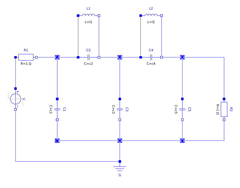
Figure 2. Graphical representation of the Cauer low-pass-filter Modelica.Electrical.Analog.Examples.CauerLowPassAnalog.

has structural singularities.

To produce a complete and consistent set of initial conditions for the DAE, exporting tools usually use a symbolic index reduction algorithm.

The model has nine state candidates

1: L1.v (unit = "V" stateSelect=StateSelect.never ) "Voltage drop of the two pins (= p.v - n.v)" type: Real
2: L2.v (unit = "V" stateSelect=StateSelect.never ) "Voltage drop of the two pins (= p.v - n.v)" type: Real
3: C2.v (start = 0.0 unit = "V" ) "Voltage drop of the two pins (= p.v - n.v)" type: Real
4: C4.v (start = 0.0 unit = "V" ) "Voltage drop of the two pins (= p.v - n.v)" type: Real
5: L1.i (start = 0.0 unit = "A" fixed = true ) "Current flowing from pin p to pin n" type: Real
6: L2.i (start = 0.0 unit = "A" fixed = true ) "Current flowing from pin p to pin n" type: Real
7: C1.v (start = 0.0 unit = "V" fixed = true ) "Voltage drop of the two pins (= p.v - n.v)" type: Real
8: C5.v (start = 0.0 unit = "V" fixed = true ) "Voltage drop of the two pins (= p.v - n.v)" type: Real
9: C3.v (start = 0.0 unit = "V" fixed = true ) "Voltage drop of the two pins (= p.v - n.v)" type: Real

and four constraint equations

1: L2.v = C3.v - C5.v
2: L1.v = C1.v - C3.v
3: C4.v = L2.v
4: C2.v = L1.v

Modelica tools that want to export an ODE ModelExchange FMU need to reduce the perturbation index to index 1 to end up with an ODE representation of the DAE system.

One option to achieve this is the so called dummy derivative method. From the set of state candidates, five state variables are chosen (e.g. C1.v, C3.v, C5.v, L1.i, L2.i) and the constraint equations

\[\begin{split} C2.v &= L1.v \\ L1.v &= C1.v - C3.v \\ C4.v &= L2.v \\ L2.v &= C3.v - C5.v \end{split}\]

are differentiated

\[\begin{split} \frac{d}{dt}C2.v &= \frac{d}{dt}L1.v \\ \frac{d}{dt}L1.v &= \frac{d}{dt}C1.v - \frac{d}{dt}C3.v \\ \frac{d}{dt}C4.v &= \frac{d}{dt}L2.v \\ \frac{d}{dt}L2.v &= \frac{d}{dt}C3.v - \frac{d}{dt}C5.v \end{split}\]

which results in four additional dummy states ($DER.L1.v, $DER.L2.v, $DER.C2.v, $DER.C4.v). Here the Modelica keyword stateSelect influences how variables are picked.

3.1.2. Scaling Power Grids Example

For simulation models representing power grids on a national or larger scale, traditional ODE solvers could struggle with convergence and performance. Also, the time needed to perform symbolic transformation from DAE to ODE is growing with the number of equations.

See for example Modelica models ScalableTestSuite.Electrical.TransmissionLine.ScaledExperiments.TransmissionLineModelica_N_10 to ScalableTestSuite.Electrical.TransmissionLine.ScaledExperiments.TransmissionLineModelica_N_1280 from ScalableTestSuite ^[4].

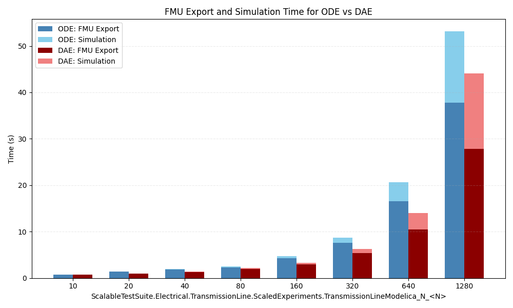
The simulation was performed using OpenModelica v1.27-dev-92 with the following settings:

DAE export: --daeMode
Method: Sundials IDA ^[5]

Since OpenModelica does not support FMI 3.0 or FMI-LS-DAE at the time of writing, the export and simulation times were measured using OpenModelica’s default C export and simulation.

4. Layered Standard Manifest File

This layered standard requires the use of a layered standard manifest file and it shall be stored inside the FMU at the following path: /extra/org.fmi-standard.fmi-ls-dae/fmi-ls-manifest.xml.

[Add figure here] shows the root element fmi-ls-dae.

Three additional elements - <EnableDAE>, <AlgebraicVariables>, and <ModelStructure> - are included as direct children of the root element in the layered standard manifest file to describe the DAE formulation.

Table 3. `fmi-ls-dae` child elements.
Element	Description
`<EnableDAE>`	Required element referencing the structural parameter in `modelDescription.xml` that enables DAE mode.
`<AlgebraicVariables>`	List of all algebraic variables exposed for the DAE formulation.
`<ModelStructure>`	Defines the structure of the DAE formulation for the model. Especially, the ordered lists of outputs, continuous-time state, and the initial unknowns (the unknowns during InitializationMode) are re-defined and overwrite the corresponding ModelStructure present in the `modelDescription.xml`, with the addition of the residuals element. The algebraic variables can now also be included as dependencies.
Section 4.4	Optional annotations for the top-level element.

The XML attributes of <fmi-ls-dae> are:

Table 4. `<fmi-ls-dae>` attribute details.
Attribute	Namespace	Value	Description
`fmi-ls-name`	`http://fmi-standard.org/fmi-ls-manifest`	`org.fmi-standard.fmi-ls-dae`	Name of the layered standard in reverse domain name notation.
`fmi-ls-version`	`http://fmi-standard.org/fmi-ls-manifest`	`0.1.0`	Version of the layered standard. This layered standard uses semantic versioning, as defined in [PW13].
`fmi-ls-description`	`http://fmi-standard.org/fmi-ls-manifest`	`Layered standard for DAE support in FMI.`	String with a brief description of the layered standard that is suitable for display to users.

4.1. Enabling DAE mode

The element <EnableDAE> references the structural parameter in the modelDescription.xml that enables DAE mode. See Section 2.2.1 for the full semantics and the calling sequences used to change the mode.

Table 5. Attributes to `<EnableDAE>` element.
Attribute	Description
`valueReference`	The value reference of the structural parameter present in the `ModelVariables` of the `modelDescription.xml` that enables DAE mode.

4.2. Algebraic variables

The element <AlgebraicVariables> defines the list of the algebraic variables.

Table 6. AlgebraicVariables elements.
Element	Description
`AlgebraicVariable`	An `<AlgebraicVariable>` present in the `ModelVariables` element of the modelDescription.xml.

Each <AlgebraicVariable> has only one attribute defining the value reference.

Table 7. Attributes to `<AlgebraicVariable>` element.
Attribute	Description
`valueReference`	The value reference for the algebraic variable present in the `ModelVariables` of the modelDescription.xml.

4.3. Model Structure

The structure of the model for the DAE-formulation is defined in element <ModelStructure>. It defines the dependencies between variables. The <ModelStructure> element is extended with an additional element - <Residual> - and the optional dependencies can now include algebraic variables.

An FMU that follows this layered standard must expose all residuals with the <Residual>.

The <ModelStructure> defined here extends the one from the core FMI standard. All elements defined there (Output, ContinuousStateDerivative, ClockedState, InitialUnknown, EventIndicator) retain their existing semantics, with the addition that each element’s dependencies attribute may now also reference algebraic variables.

The <ModelStructure> element is extended with one additional element, <Residual>, described below.

Table 8. Additional ModelStructure element.
Element	Description
`Residual`	Ordered list of residual equations (constraints). Each `<Residual>` contains one or more `<Formulation>` child elements. When a single `<Formulation>` is present, it defines the residual equation directly. When multiple `<Formulation>` elements are present within the same `<Residual>`, they represent the same constraint differentiated to successive orders. This grouping tells the importer that the equations are structurally related, which can e.g. be used to perform index reduction with dummy derivatives or projection methods. Note that each formulation inside one residual element must reference unique variables in the FMU. The functional dependency is defined as: ${0 := \mathbf{f}_{\mathit{res}}(\mathbf{x}_c, \mathbf{z}_c, \mathbf{u}_c, t, \mathbf{p})}$

4.3.1. Formulation

Each <Formulation> element within a <Residual> has the following attributes:

Table 9. Attributes to `<Formulation>` element.
Attribute	Description
`valueReference`	The value reference of the residual variable ${v_{\mathit{unknown}}}$, which must be present in the `ModelVariables` element of the `modelDescription.xml`.
`index`	Optional attribute indicating the DAE index of the original constraint, i.e., how many times this particular equation needs to be differentiated in order to solve for a particular derivative.
`dependencies`	Optional attribute defining the algebraic dependencies as a list of value references of the knowns ${\mathbf{v}_{\mathit{known}}}$ that this formulation directly depends on. Knowns ${\mathbf{v}_{\mathit{known}}}$ in ContinuousTimeMode (ME) for `<Formulation>` elements are: inputs (variables with causality = input), continuous states, continuous state derivatives, parameters (variables with causality = parameter), algebraic variables (variables listed in the `<AlgebraicVariables>` element), independent variable (usually time; causality = independent). If `dependencies` is not present, it must be assumed that the formulation depends on all knowns. If `dependencies` is present as an empty list, the formulation depends on none of the knowns. Otherwise the formulation depends on the knowns defined by the given value references.
`dependenciesKind`	See the description of `dependenciesKind` in the core FMI standard. TODO: Extend to help importer?

4.4. Annotations

TODO

4.5. Getting Partial Derivatives

The partial derivative API functions fmi3GetDirectionalDerivative and fmi3GetAdjointDerivative are used as defined in the core FMI standard, with the following extensions for DAE FMUs:

Algebraic variables (variables listed in <AlgebraicVariables>) could appear as knowns for any unknown.
When the unknown is a <Formulation> in a <Residual>(i.e., a residual variable), continuous state derivatives could additionally appear as knowns.

4.6. Hello World DAE Example

Below outlines how to map the different forms of the Hello World DAE Example to the manifest file detailed here.

4.6.1. Hello World DAE - Fully-Implicit DAE

The fully-implicit representation

\[F(\dot{x}, x, t) = 0\]

is given by

\[F: \mathbb{R}^3 \times \mathbb{R}^3 \times \mathbb{R} \to \mathbb{R}^3, \begin{pmatrix} x \\ \dot{x} \\ t \end{pmatrix} \mapsto \begin{pmatrix} F_1 \\ F_2 \\ F_3 \end{pmatrix} = \begin{pmatrix} \dot{x_1} - x_2 \\ x_2 + 2 x_3 - x_1 \\ x_2 - 3 x_3 - 2 x_1 \end{pmatrix}\]

Assume the FMU has these variables:

Variable	valueReference
$t$	1
$x_1$	2
$x_2$	3
$x_3$	4
$\dot{x_1}$	5
$\dot{x_2}$	6
$\dot{x_3}$	7
$F_1$	8
$F_2$	9
$F_3$	10

In this case x_2 and x_3 do not appear differentiated in any equations, hence they are classified as algebraic (element of <AlgebraicVariables>). An example of the <AlgebraicVariables> and <ModelStructure> elements would be:

<AlgebraicVariables>
  <AlgebraicVariable valueReference="3"/> <!-- x_2 -->
  <AlgebraicVariable valueReference="4"/> <!-- x_3 -->
</AlgebraicVariables>
<ModelStructure>
  <Residual> <!-- F1 -->
    <Formulation
      valueReference="8"
      dependencies="5 3"
      dependenciesKind="fixed fixed"/>
  </Residual>
  <Residual> <!-- F2 -->
    <Formulation
      valueReference="9"
      dependencies="2 3 4"
      dependenciesKind="fixed fixed fixed"/>
  </Residual>
  <Residual> <!-- F3 -->
    <Formulation
      valueReference="10"
      dependencies="2 3 4"
      dependenciesKind="fixed fixed fixed"/>
  </Residual>
</ModelStructure>

The derivatives of x_1, x_2, and x_3 (\dot{x_1}, \dot{x_2}, \dot{x_3}) are still noted with the derivative attribute under the ModelVariables element, which gives the importer all the information they need to solve the equations.

4.6.2. Hello World DAE - Semi-Explicit DAE

The semi-explicit representation

\[\begin{split} \dot{x} & = f(x, y, t) \\ 0 & = g(x, y, t) \end{split}\]

is given by

Assume the FMU has the following variables:

Variable	valueReference
$t$	1
$x$	2
$y_1$	3
$y_2$	4
$\dot{x}$	5
$g_1$	6
$g_2$	7

This case contains the same algebraic variables. However this time the the derivative of x is given in explicit form in the ModelStructure:

<AlgebraicVariables>
  <AlgebraicVariable valueReference="3"/> <!-- y1 -->
  <AlgebraicVariable valueReference="4"/> <!-- y2 -->
</AlgebraicVariables>

<ModelStructure>
  <ContinuousStateDerivative
    valueReference="5"
    dependencies="3"
    dependenciesKind="fixed"/> <!-- dot(x) = y1 -->
  <Residual> <!-- g1: y1 + 2*y2 - x = 0 -->
    <Formulation
      valueReference="6"
      dependencies="2 3 4"
      dependenciesKind="fixed fixed fixed"/>
  </Residual>
  <Residual> <!-- g2: y1 - 3*y2 - 2*x = 0 -->
    <Formulation
      valueReference="7"
      dependencies="2 3 4"
      dependenciesKind="fixed fixed fixed"/>
  </Residual>
</ModelStructure>

4.6.3. Hello World DAE - Explicit ODE

This simple system could also be transformed into an explicit ODE formulation

\[\begin{split} \dot{x} &= \frac{7}{5}x \end{split}\]

with local variables $y$ and $z$

\[\begin{split} y &= \frac{7}{5}x \\ z &= -\frac{x}{5} \end{split}\]

and exported as an ODE ModelExchange FMU:

Variable	valueReference
$t$	1
$x$	2
$y$	3
$z$	4
$\dot{x}$	5

This would correspond to the regular ODE ModelStructure:

<ModelStructure>
  <ContinuousStateDerivative <!-- dot(x) = 7/5 * x -->
    valueReference="5"
    dependencies="2"
    dependenciesKind="fixed"/>
</ModelStructure>

4.7. Example 2 (differentiated formulations)

Consider the following index 2 DAE system:

$r_1 = C_1\frac{dx_1}{dt} + y = 0$

$r_2 = C_2\frac{dx_2}{dt} - y + 1 = 0$

$r_3 = x_1 - x_2 = 0$

Assume it is exported as a DAE FMU with the following variables:

Variable	valueReference
$x_1$	1
$x_2$	2
$y$	3
$\frac{dx_1}{dt}$	4
$\frac{dx_2}{dt}$	5
$r_1$	6
$r_2$	7
$r_3$	8
$\frac{dr_3}{dt}$	9

Case 1: No structural analysis. The importer is responsible to figure out how to solve the system:

<ModelStructure>
  <Residual> <!-- r1 -->
    <Formulation
      valueReference="6"
      dependencies="3 4"
      dependenciesKind="dependent dependent"/>
  </Residual>
  <Residual> <!-- r2 -->
    <Formulation
      valueReference="7"
      dependencies="3 5"
      dependenciesKind="dependent dependent"/>
  </Residual>
  <Residual> <!-- r3 -->
    <Formulation
      valueReference="8"
      dependencies="1 2"
      dependenciesKind="dependent dependent"/>
  </Residual>
</ModelStructure>

Case 2: The FMU additionally indicates that $r_3$ is a constraint of index 2, i.e., it needs to be be differentiated twice to obtain an index 1 system. This gives the importer structural information to know to apply a solver able to handle index 2 problems:

<ModelStructure>
  <Residual> <!-- r1 -->
    <Formulation
      valueReference="6"
      dependencies="3 4"
      dependenciesKind="dependent dependent"/>
  </Residual>
  <Residual> <!-- r2 -->
    <Formulation
      valueReference="7"
      dependencies="3 5"
      dependenciesKind="dependent dependent"/>
  </Residual>
  <Residual> <!-- r3, index=2 signals this constraint needs 2 differentiations -->
    <Formulation
      index="2"
      valueReference="8"
      dependencies="1 2"
      dependenciesKind="dependent dependent"/>
  </Residual>
</ModelStructure>

Case 3: The FMU exposes both $r_3$ and its time derivative $\dot{r}_3$ grouped within the same <Residual>, which indicates that these are the original constraint and its differentiated form. The importer can use this grouping to apply the dummy derivatives algorithm or use $r_3$ as a drift-correction projection when integrating the index 1 formulation:

$r_3 = x_1 - x_2 = 0$

$\dot{r}_3 = \frac{dx_1}{dt} - \frac{dx_2}{dt} = 0$

<ModelStructure>
  <Residual> <!-- r1 -->
    <Formulation
      valueReference="6"
      dependencies="3 4"
      dependenciesKind="dependent dependent"/>
  </Residual>
  <Residual> <!-- r2 -->
    <Formulation
      valueReference="7"
      dependencies="3 5"
      dependenciesKind="dependent dependent"/>
  </Residual>
  <Residual> <!-- r3 and its derivative, grouped as related formulations -->
    <Formulation
      index="2"
      valueReference="8"
      dependencies="1 2"
      dependenciesKind="dependent dependent"/> <!-- r3 -->
    <Formulation
      index="1"
      valueReference="9"
      dependencies="4 5"
      dependenciesKind="dependent dependent"/> <!-- der(r3) -->
  </Residual>
</ModelStructure>

The API for partial derivative, GetDirectionalDerivative and/or GetAdjointDerivative could be used with this structure to apply the dummy derivatives algorithm, or the index 2 constraint can serve as a projection constraint when integrating the index 1 formulation.

References

[cui2020mass] Cui, Hantao, Fangxing Li, and Joe H. Chow. "Mass-matrix differential-algebraic equation formulation for transient stability simulation." arXiv preprint arXiv:2008.03883, 2020.

[cellier2006continuous] Cellier, François E., and Ernesto Kofman. "Continuous system simulation". Boston, MA: Springer US, 2006.

[hairer2006numerical] Hairer, Ernst, Christian Lubich, and Michel Roche. "The numerical solution of differential-algebraic systems by Runge-Kutta methods". Vol. 1409. Springer, 2006.

[cellier1993automated] Cellier, Francois E., and Hilding Elmqvist. "Automated formula manipulation supports object-oriented continuous-system modeling". IEEE Control Systems Magazine 13.2 (1993): 28-38.
[braun2017solving] Willi Braun, Francesco Casella, and Bernhard Bachmann. "Solving Large-Scale Modelica Models: New Approaches and Experimental Results Using OpenModelica". Linköping Electronic Conference Proceedings (Print), pp. 557-563. Linköping University Electronic Press, 2017. https://re.public.polimi.it/bitstream/11311/1065357/1/2017-BraunCasellaBachmann.pdf

[casella2015simulation] Casella, Francesco. "Simulation of Large-Scale Models in Modelica: State of the Art and Future Perspectives". Proceedings of the 11th International Modelica Conference, pp. 459-468, 2015. https://dx.doi.org/10.3384/ecp15118459
[PW13] Preston-Werner, T. (2013): Semantic Versioning 2.0.0. https://semver.org/spec/v2.0.0.html

1. Source: https://en.wikipedia.org/wiki/Differential-algebraic_system_of_equations

2. e.g. by using Pantelides algorithm, see [cellier1993automated]

3. Modelica Standard Library version 4.1.0

4. https://github.com/casella/ScalableTestSuite, see also [casella2015simulation]

5. https://computing.llnl.gov/projects/sundials/ida

Variable	valueReference
\(t\)	1
\(x_1\)	2
\(x_2\)	3
\(x_3\)	4
\(\dot{x_1}\)	5
\(\dot{x_2}\)	6
\(\dot{x_3}\)	7
\(F_1\)	8
\(F_2\)	9
\(F_3\)	10

Variable	valueReference
\(t\)	1
\(x\)	2
\(y_1\)	3
\(y_2\)	4
\(\dot{x}\)	5
\(g_1\)	6
\(g_2\)	7

Variable	valueReference
\(t\)	1
\(x\)	2
\(y\)	3
\(z\)	4
\(\dot{x}\)	5

Variable	valueReference
\(x_1\)	1
\(x_2\)	2
\(y\)	3
\(\frac{dx_1}{dt}\)	4
\(\frac{dx_2}{dt}\)	5
\(r_1\)	6
\(r_2\)	7
\(r_3\)	8
\(\frac{dr_3}{dt}\)	9

FMI Layered Standard for DAE (FMI-LS-DAE)

FMI Layered Standard for DAE (FMI-LS-DAE)

1. Introduction

1.1. Intent of this Document

1.2. How to read this Document

1.3. Overview

2. Common Concepts

2.1. Mathematical Notation

2.1.1. DAE representation

2.1.1.1. Fully-Implicit DAE

2.1.1.2. Semi-Explicit Index 1 / Hessenberg index 1 DAE

2.1.1.3. Relationship between fully-implicit and semi-explicit DAE

2.1.1.4. Semi-Explicit DAE

2.1.1.5. Mass matrix DAE

2.1.1.6. Linear time-invariant DAE

2.1.2. Indices

2.1.2.1. Differential Index

2.1.2.2. Perturbation Index

2.1.2.2.1. Example of Structural Singularity

2.1.3. Hello World DAE Example

2.1.3.1. Hello World DAE - Fully-Implicit DAE

2.1.3.2. Hello World DAE - Semi-Explicit DAE

2.1.3.3. Hello World DAE - Explicit ODE

2.2. Changing between ODE and DAE Mode

2.2.1. The enableDAEModeVariable Structural Parameter

2.2.2. Entering DAE Mode

2.2.2.1. At Instantiation (Configuration Mode)

2.2.2.2. During Simulation (Reconfiguration Mode)

3. Use Cases

3.1. Generic DAE Use Case

3.1.1. Modelica Example CauerLowPassAnalog

3.1.2. Scaling Power Grids Example

4. Layered Standard Manifest File

4.1. Enabling DAE mode

4.2. Algebraic variables

4.3. Model Structure

4.3.1. Formulation

4.4. Annotations

4.5. Getting Partial Derivatives

4.6. Hello World DAE Example

4.6.1. Hello World DAE - Fully-Implicit DAE

4.6.2. Hello World DAE - Semi-Explicit DAE

4.6.3. Hello World DAE - Explicit ODE

4.7. Example 2 (differentiated formulations)

References

2.2.1. The `enableDAEModeVariable` Structural Parameter